8/29/11
E. Brodsky and H. Kanamori
Scans of the Caltech Archive
This directory contains images of seismograms formally stored by the Caltech in the Kresge Seismological Laboratory, Pasadena CA. The images are a subset of the approximately 1 million paper records accumulated from 1928 through the mid-1980�s. The images were scanned in 2009-2010 by Google in collaboration with UC Santa Cruz as part of the Google Books project. Scans include fronts and backs of the paper records and are organized into directories that each corresponds to an individual box in which the records were originally stored at Kresge. The goal of this electronic library of seismograms is to allow users to simulate the experience of going to the paper archives and flipping through a box to find a record. The organization is imperfect and the search engine non-existent, but the original records are now as accessible to the world-wide user group as they once were to a small group of California seismologists.
As only a small part of the collection could be scanned, the images sent to Google were prioritized as follows:
1) The Special Collection was scanned in its entirety. The Special Collection contains records collected by Caltech seismologists for their study on significant historical events. These records are predominantly from the Pasadena long-period Press-Ewing seismometers, but the collection is extremely heterogeneous and includes copies of records from a number of historical sites. The Special Collection directories are labeled with brief names of important events or sites contained. Often the station information is written on the back of the record. The station information is either a station code or a pier number at Pasadena (see below).
2) The Southern California Seismic Network short-period records were scanned with highest priority going to the earliest records. Records that were deemed too brittle to run through the scan apparatus were skipped. These directories are labeled with the date range covered and the annotation �SCSN�. Within each date range, the full suite of operating instruments is covered. Usually records appear in a directory chronologically with all of the stations in a row for each day and then the same suite of stations again the next day. The station codes and dates are usually stamped on the front of the record.
User information
Each directory contains the full images numbered in the order they were removed from the box (hopefully the filing order). The directories also contain thumbnails of each image to enable faster browsing. The thumbnails have the same name as the original high-resolution file with the appendix �.thumb.jpg�. Sometimes a box was split in two due to an scanner interruption. In these cases, the two directories have the appendix �a� and �b�.
There is also a user-editable documentation tool at: /CaltechSeismoWiki/ This is meant to be a community document to help users identify events and instrumental issues. Please read the document upon starting your work and add to it as often as you can. The Wiki requires a user-account that is automatically generated if you fill in the form at: /CaltechSeismoWiki/Login.jsp?redirect=Main.
Each directory also will have a user-editable README. (This is not yet implemented). This is meant to be a community document to help users identify events and instrumental issues. Please read the document upon entering a directory and add to it when you leave.
Instrument Responses
The two most common sensor types in the archive are Wood-Anderson short-periods seismometers in the SCSN and Press-Ewing seismometers in the special collections. Typical response curves are in Figure 1 and instrument constants in Table 1. Further information is available in the Appendix to Kanamori (1988).
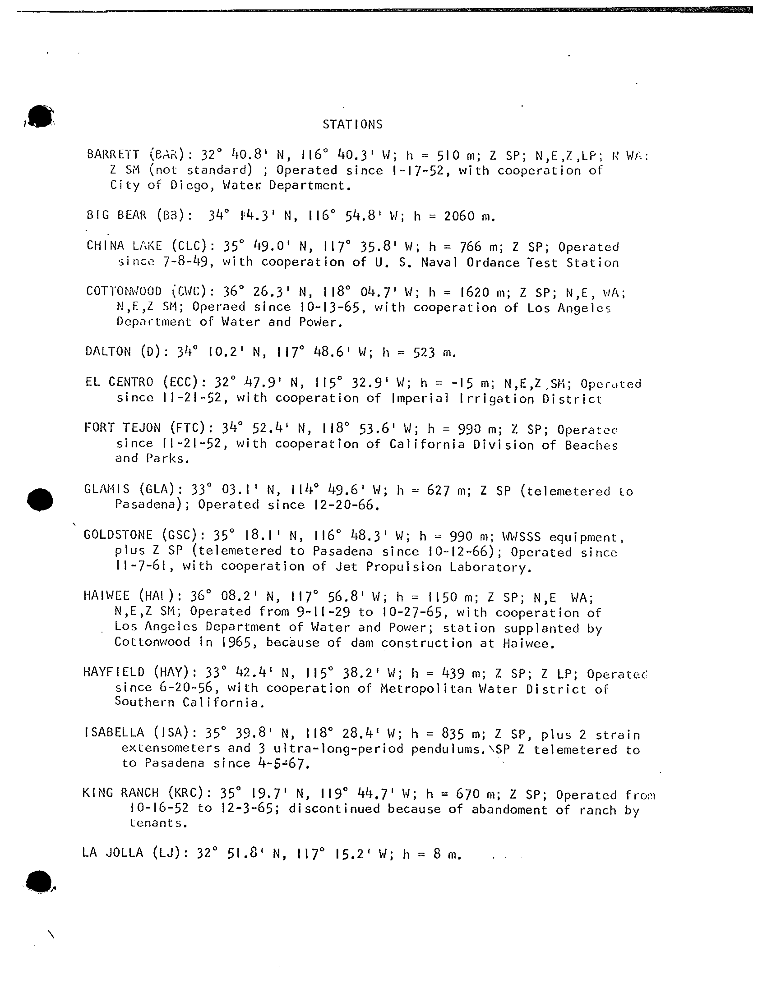
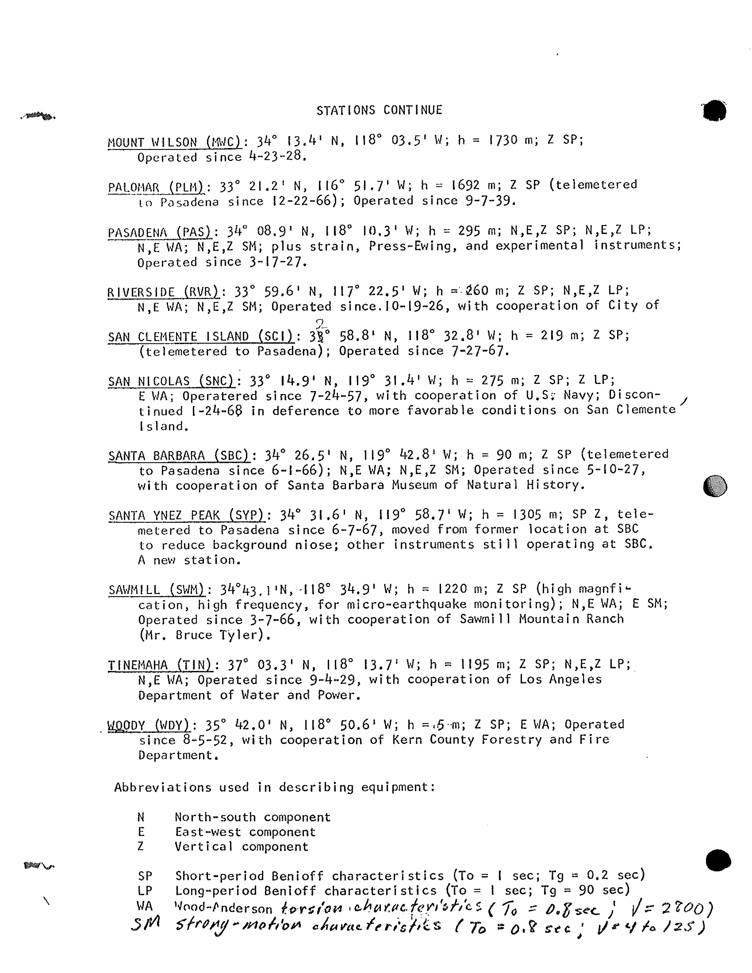
The short-period records are stamped with a station code. The SCSN stations eventually covered all of Southern California (Figure 2) and are documented in Appendix A of this document with the station names, abbreviations, coordinates, sensor types and basic operational notes.
Many of the records in the special collection are marked
with handwritten pier numbers on the reverse rather than instruments. These
numbers correspond to a specific location in the Pasadena instrument room and
the corresponding sensor changes with time. The most common pier numbers are
34A, B and C corresponding to the three components of the Press-Ewing
instruments. A map of the Kresge building with pier numbers and sensor annotations
is in Figure 3.
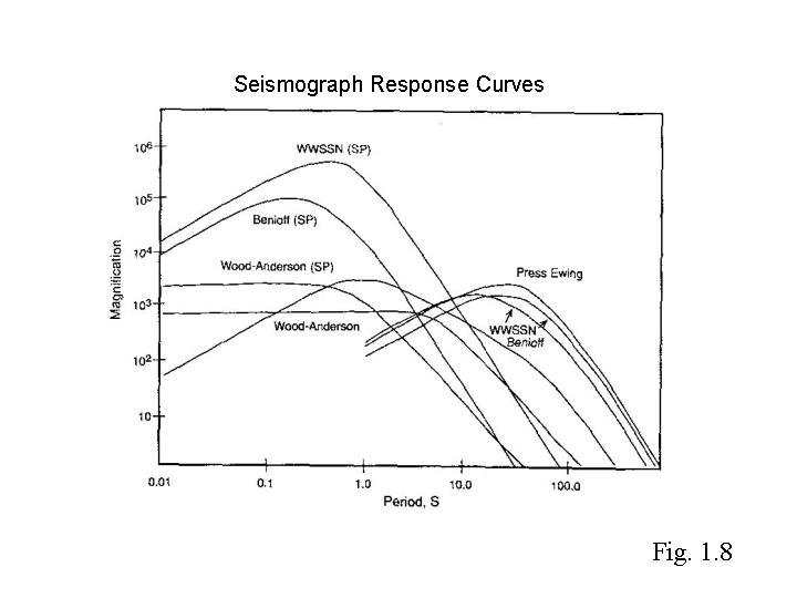
Figure 1. Approximate response curves of historical seismograms (Courtesy H. Kanamori).
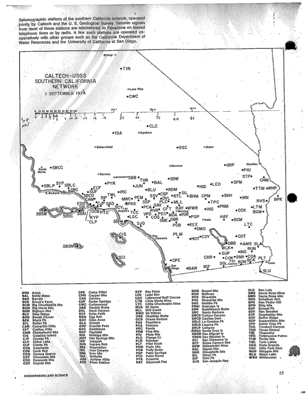
Figure 2. Map of the SCSN station configuration in 1974.
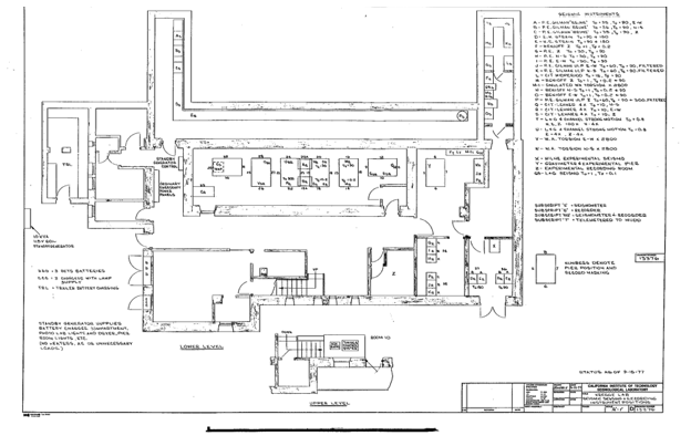
Figure 3. Kresge laboratory instrumentation
map. Use
this map to connect pier numbers to sensor types.
Typical Seismograph Constants
|
Seismograph |
Ts
(sec) |
hs |
Tg
(sec) |
hg
|
σ2 |
V(1) |
||||||
|
Wood-Anderson
(standard) |
0.8 |
0.8 |
NA |
NA
|
NA |
2800(2) |
||||||
|
Press-Ewing
|
30 |
1 |
90 |
1 |
0.1 |
2300(3) |
||||||
|
Benioff (SP) |
1.0
|
1 |
0.2 |
1 |
0.1 |
100,000(3) |
||||||
|
Benioff (LP)
|
1.0
|
1 |
90
|
1 |
0.1 |
3000(3) |
|
|||||
|
WWSSN
(SP)
|
1.0
|
1 |
0.7
|
1 |
0.1 |
50,000(4) |
|
|||||
|
WWSSN
(LP1)
|
15
|
1 |
100
|
1 |
0.1 |
1500(5) |
|
|||||
|
WWSSN
(LP2) |
30
|
1.75 |
100
|
1 |
0.1
|
1500(5) |
||||||
Table
1. Summary of the constants for typical seismographs often
used. Here, Ts, hs, Tg, hg, σ2, and V are the pendulum period,
damping constant of the pendulum, galvanometer period, damping constant of the galvanometer,
coupling factor, and the magnification.
The values listed are nominal values frequently used. However, the actual values may differ
considerably from these.
Notes:
(1) V
varies for different stations.
(2) Sometimes
2080 is used.
(3) The
magnification at the peak of the response.
(4) The
magnification at the period of 1 s.
(5) The
magnification at the period of the pendulum.
For the computation of the
Wood-Anderson response, see Richter (1958). For others, see Hagiwara (1958).
References
Hagiwara, T., A note of the theory of the electromagnetic seismograph. Bulletin of the Earthquake Research Institute. 36, 139-164, 1958.
Kanamori, H. Importance of Historical Seismograms for Geophysical Research in Historical Seismograms and Earthquakes of the World, eds., Lee, Meyers, and Shimazaki, Academic Press, 1988.
Richter, C.F. Elementary Seismology, W.H. Freeman and Company, 1958.
Appendix A