Overview

In addition to being able to read and write SAC data files in one's own C or FORTRAN programs (see SAC Reading and Writing Routines ), one can use many of SAC's data-processing routines in stand-alone codes. The internal routines here are wrapped in an interface that should be more streamlined to use than previous versions to v102.0. The libraries libsac.a and libsacio.a are in ${SACHOME}/lib.

For more detailed examples, see ${SACHOME}/doc/examples contained in the SAC distribution.

Callable in C and Fortran

All of these available functions are simplified wrappers around internally used functions within SAC with obscure, shortened and forgotten names and extra, usually unneeded, or confusing parameters. Each function documented below should be callable directly from C and Fortran. The Fortran wrappers should work simply for Fortan compilers that append underscores to function names internally within the program.

A difference between the C and Fortran versions is the calling convention of pass-by-value (default in C) and pass-by-reference (Fortran).

Compiling

To ease the requirements for compilation and linking, a helper script is provided, ${SACHOME}/bin/sac-config, which should output the necessary flags and libraries for SAC. If you have the a C compiler or a Fortran compilers, try:

cc -o program main.c subs.c `sac-config --cflags --libs libsac libsacio`

gfortran -o program main.f `sac-config --cflags --libs libsac libsacio`

Fourier Transform (FFT)

Given below are both single- and double-precision routines for doing forward and inverse Fourier transforms. All transforms are performed in double precision, as all subroutine calls within SAC use the same internal code path. Single-precision versions internally convert/copy the input arrays to double recision as a prelude to perfomring the transform, and the results are then converted back to single precision on return. The internal calculations are done using a power-of-2 number of points. For a forward transform, n need not be a power of 2, but the output nf must be the next power of 2 greater than or equal to n. Parameter nf must be defined prior to calling any of these routines.

// Forward Transform - Single Precision
void   fft (float data, int n, float *re, float *im, int nf)
void   fftz(float data, int n, float complex *z, int nf)

// Forward Transform - Double Precision
void  dfft (double data, int n, double *re, double *im, int nf)
void  dfftz(double data, int n, double complex *z, int nf)

// Inverse Transform - Single Precision
void   ifft(float data, int n, float *re, float *im, int nf)
void  ifftz(float data, int n, float complex *z, int nf)

// Inverse Transform - Double Precision
void  idfft(double data, int n, double *re, double *im, int nf)
void idfftz(double data, int n, double complex *z, int nf)

Compute the Fourier Transform (or inverse transform) of a data series.

Arguments

• data - Input time series for forward transform; output time series for inverse
• n - Length of time series on input for forward transform; number of points desired from the inverse transform
• z - Complex FFT Spectrum
• re - Real Component of the Fourier spectrum; calculated in forward transform, input for inverse transform.
• im - Imaginary Component of the Fourier spectrum.
• nf - Input length of re, im, and z for inverse transform; calculated in forward transform.

Normalization

Normalization of the transform by the length, nf, is done on the inverse transforms

Time Scaling

Time scaling is not performed within these functions, but can be accomplished by multiplying the Fourier spectrum by the sampling rate, dt. If the scaling is applied to the spectrum, make sure to remove the time shift to get back to the original time series.

Frequency Ordering

Amplitudes are ordered frequency starting with the zero frequency, through positive frequencys to the Nyquist df*(nf/2), then backwards through the negative frequencies

0, df, ... , df*(nf/2-1), df*(nf/2), -df*(nf/2-1), ... , -df

Examples

integer n, nf
real*8 :: data(16), data2(16)
real*8 :: re(64), im(64)
complex*16 :: z(16)

n  = 10

! Find next power of 2
nf = 4
do while (nf < n)
   nf = nf * 2
enddo

! FFT with real/imaginary
call dfft(data, n, re, im, nf)
call idfft(data2, n, re, im, nf)

! FFT with complex number
call dfftz(data, n, z, nf)
call idfftz(data2, n, z, nf)

Remove Mean

void remove_mean (float *data, int n)

Remove the mean of a data series. The mean of the data series is automatically calculated and removed from the data series.

Arguments

• data - Input data series
• n - length of data

Note: Data is modified in place.

Examples

implicit none

integer,parameter :: nmax = 1776
integer :: npts, nerr
real*4 :: data(nmax), beg, dt

! Read in the data file
call rsac1('raw.sac', data, npts, beg, dt, nmax, nerr)

! Remove the mean of the data in place
call remove_mean(data, npts)

Effective SAC Commands

SAC> read raw.sac
SAC> rmean

Remove Trend

void remove_trend(float *data, int n, float delta, float b)

Removse the trend (along with the mean) of a data series in memory

Arguments

• data - Input data series, overwritten on output
• n - length of data
• delta - Time sampling of the data
• b - Initial time value of the data series

Note: Data is modified in place.

This calls internal rountines lifite() and rtrend().

Trend is removed as

y[i] = y[i] - yint - slope * (b + delta * i)

where y is the data

Examples

#define NMAX 1969

float y[NMAX], b, dt;
int nmax = NMAX;
int n, nerr;

// Read in the data file
rsac1("raw.sac", y, &n, &b, &dt, &nmax, &nerr, -1);

// Remove the trend of the data in place
remove_trend(y, n, dt, b);

Effective SAC Commands

SAC> read raw.sac
SAC> rtrend verbose

Filtering

Data is filtered using an Infinite Impulse Repsonse Filter. See the BANDPASS command for definitions of the filter parameters and descriptions on how to use them.

void bandpass(float *data, int n, float dt, float low, float high)
void lowpass(float *data, int n, float dt, float corner)
void highpass(float *data, int n, float dt, float corner)

void filter(int prototype,
            int type,
            float *data, int n, float dt,
            float low, float high, int passes, int order,
            float transition,
            float attenuation)

Arguments

• data - Input and output data
• n - Length of data
• dt - Time sampling of the data (seconds)
• low - low frequency corner
• high - high frequency corner
• corner - corner of the filter for lowpass or highpass

• passes - Number of passes

  • 1 - forward pass only (causal)
  • 2 - forward and backward pass (zero-phase)

• order - Filter Order, not to exceed 10, 4-5 should be sufficient
• transition - Transition Bandwidth, only used in Chebyshev Type I and II Filters
• attenuation - Attenuation factor, amplitude reached at stopband edge, only used in Chebyshev Type I and II Filters

• prototype - Filter Prototype

  • 0 - Butterworth filter
  • 1 - Bessel filter
  • 2 - Chebyshev Type I filter
  • 3 - Chebyshev Type II filter

• type - Filter Type

  • 0 - Bandpass
  • 1 - Highpass
  • 2 - Lowpass
  • 3 - Bandreject

Examples

Bandpass filter in C

 #define NMAX 2015
 float y[NMAX], b, dt;
 int n, nerr, nmax = NMAX;

 // Read in the data file
 rsac1("raw.sac", y, &n, &b, &dt, &nmax, &nerr, -1);

 // bandpass filter from 0.10 Hz to 1.00 Hz
 bandpass(y, n, dt, 0.10, 1.00);

Highpass filter in Fortran

  implicit none
  integer nmax, n, nerr, sac_compare
  real*4 :: y(2012), b, dt
  nmax = 2012

  ! Read in the data file
  call rsac1("raw.sac", y, n, b, dt, nmax, nerr)

  ! highpass filter at 10.0 Hz
  call highpass(y, n, dt, 10.0)

**Effective SAC Commands**

SAC> read raw.sac
SAC> bp co 0.10 1.0 p 2 n 4

SAC> read raw.sac
SAC> hp co 10.0 p 2 n 4

Further examples are given in ${SACHOME}/doc/examples/filter/ . Because one uses FFT that pads with zeros, it is often prudent to precede the filter with rtrend ; taper.

Cross Correlation

void correlate(float *f, int nf, float *g, int ng, float *c, int nc)

Compute the cross-correlation of two signals

Arguments

• f - First time series
• nf - Length of first time series
• g - Second time series
• ng - Length of second time series
• c - Cross correlation time series
• nc - Size of c, must be at least (nf + ng - 1)

Return: Cross correlation function, length: nf + ng - 1

If the signals are not the same length, then find the longest signal, make both signals that length by filling the remainder with zeros (pad at the end) and then run them through crscor

Examples

Effective SAC Commands

SAC> read file1.sac file2.sac
SAC> correlate

Cross Correlation Extras

int correlate_max(float *c, int nc)

Find the maximum of a correlation

Arguments

• c - float array (returned from correlate function)
• nc - length of c

Return: Index of maximum value in array

float correlate_time(float dt, float b, int i)

Compute the time of a data point given dt and begin time

Arguments

• dt - Time sampling
• b - Begin time
• i - data sample

Return: time value (b + i * dt)

float * correlate_time_array(float dt, float b, int n)

Compute a time array given dt and begin time

Arguments

• dt - Time sampling
• b - Begin time
• n - Length of data array

Return: time array

float correlate_time_begin(float dt, float n1, float _n2, float b1, float b2)

Compute begin time from a corealtion of two time series

Arguments

• dt - Time sampling
• n1 - Length of first time series
• n2 - Length of second time series (unused)
• b1 - Begin time of first time series
• b2 - Begin time of second time series

Return: -dt * (n1 - 1) + (b2 - b1)

This accounts for the possible differences in begin times of two time series

Envelope Calculation

void envelope(int n, float *in, float *out)

Compute the envelope of a time series using the Hilbert transform

Arguments

• n - Length of input and output time series
• in - Input time series
• out - Output time series with envelope applied

The envelope is applied as such where the H(x) is the Hilbert transform:

out = sqrt( H( in(t) )^2 + in(t)^2 )

Examples

#define NMAX 1929
int nlen, nerr, nmax;
float yarray[NMAX], yenv[NMAX];
float beg, delta;

nmax = NMAX;

// Read in data file
rsac1("raw.sac", yarray, &nlen, &beg, &delta, &nmax, &nerr, SAC_STRING_LENGTH);

// Calculate Envelope of data
envelope(nlen, yarray, yenv);

Effective SAC Commands

SAC> read raw.sac
SAC> envelope

Because one uses FFT that pads with zeros, it is often prudent to precede the filter with rtrend ; taper.

Differentiate

void dif2(float *array, int n, double delta, float *output)

Differentiate a data set using a two point differentiation

Arguments

• array - Input data to differentiate
• n - length of ararry
• delta - Time sampling of input data
• output - Output differentiated data, length n-1

This is the default scheme in the SAC program.

The output array will be 1 data point less than the input array.

Since this is not a centered differeniation, there is an implied shift in the independent variable by half the delta:

b_new = b_old + 0.5 * delta

Differntiation is performed as:

out[i] = (1/delta) * (in[i+1] - in[i])

Examples

integer,parameter :: nmax = 1000000
integer :: npts, nerr
real*4 :: data(nmax), out(nmax)
real*4 :: beg, dt

! Read in the data file
call rsac1("raw.sac", data, npts, beg, dt, nmax, nerr)

! Differentiate the data
call dif2(data, npts, dble(dt), out)

bnew = beg + 0.5 * delta
npts_new = npts - 1

Effective SAC Commands

SAC> read raw.sac
SAC> dif

Integerate

void int_trap(float *y, int n, double delta)

Integrate a data series using the trapezodial method

Arguments

• y - Input data series, overwritten on output
• n - length of y
• delta - time sampling of the data series

Integration is performed as:

out[i] = out[i-1] + (delta/2) * (in[i] + in[i+1])

where the initial out value is 0.0.

The number of points on output should be reduced by 1

len(out) = len(in) - 1

and the beging value is shifted by 0.5 delta:

b_out = b_in + 0.5 * delta

Examples

#define NMAX 2012
float y[NMAX], b, dt;
int n, nerr, nmax = NMAX;

rsac1("raw.sac", y, &n, &b, &dt, &nmax, &nerr, -1);

int_trap(y, n, (double)dt);

Effective SAC Commands

SAC> read raw.sac
SAC> int

Taper Data

// Taper using points
void taper_points(float *data, int n, int taper_type, int ipts)
void taper(float *data, int n, int taper_type, int ipts)

// Taper using a duration in seconds
void taper_seconds(float *data, int n, int taper_type, float sec, float
delta)

// Taper using a percent of the data
void taper_width(float *data, int n, int taper_type, float width)

Arguments

• data - Input data series, overwritten on output

• n - Length of data

• taper_type - Type of Taper

  • 1 - Cosine - SAC_TAPER_COSINE
  • 2 - Hanning - SAC_TAPER_HANNING [Default in SAC]
  • 3 - Hamming - SAC_TAPER_HAMMING

• ipts - Points to use in the taper

• sec - Duration of the taper in seconds

• delta - Delta of the data

• width - Percent of the data to taper [SAC default is 5%]

Examples

#define MAX 1984
float data[MAX];
int nmax, npts, nerr, taper_type;
float beg, dt, width;

nmax = MAX;

// Read in the data file
rsac1("raw.sac", data, &npts, &beg, &dt, &nmax, &nerr, -1);

// Set up taper parameters
width = 0.05;    // Width to taper original data
taper_type = 2;  // HANNING taper

taper_width(data, npts, taper_type, width);

Effective SAC Commands

SAC> read raw.sac
SAC> taper TYPE HANNING WIDTH 0.05
(these are the defaults for taper in SAC)

Cut Data

void cut(float *y, int npts, float b, float dt,
         float begin_cut, float end_cut, int cuterr,
         float *out, int *nout)

Cut a time series at specified begin and end times

Arguments

• y - Input data to be cut

• npts - Length of y

• b - Begin time of data

• dt - time sampling (seconds)

• begin_cut - Start time of cut

• end_cut - End time of cut

• cuterr -

  • 1 - Fatal - SAC_CUT_FATAL
  • 2 - Use B and E Values - SAC_CUT_USEBE
  • 3 - Fill with Zeros - SAC_CUT_FILLZ

• out - Cut data on output

• nout - Length of out

Examples

integer,parameter :: nmax = 1776
real*4 :: y(nmax), out(nmax), b, dt, cutb, cute
integer :: nerr, n, nout

max = nmax
! Read in data
call rsac1("raw.sac", y, n, b, dt, max, nerr)

nout = max
cutb = 10.0
cute = 15.0
! Cut data from 10 to 15 or from B to E if window is too big
call cut(y, n, b, dt, cutb, cute, CUT_USEBE, out, nout)

Effective SAC Commands

SAC> read raw.sac
SAC> cut 10 15
SAC> read raw.sac

See ${SACHOME}/doc/examples/create_compare/ for an example.

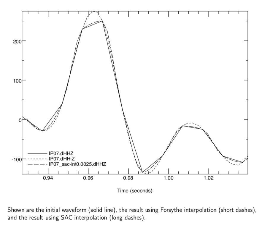
Interpolation using cubic splines

In the pre-digital-data era, data extremes were relatively easy to see because the pen or light-beam velocity went to zero at them. The interpolation scheme used by the SAC interpolate routine uses a method popularized by Wiggins that took advantage of that feature so that cycle extrema could be at digitized points.

With digital data, the extrema may not be at digitized points, and for some studies it is desirable to get a better estimate of the maxima and minima (for example, estimating magnitudes based on amplitudes or when using amplitude ratios in focal-mechanism determinations. The routine below uses a pure cubic-spline interpolation published by Forsythe, et al., that can give significantly different results from a Wiggins interpolation. The program is in in ${SACHOME}/doc/examples/interpolate. The script run_interpolate.sh shows how the interpolation program is built and run, along with how interpolation would be accomplished in SAC.

The plot below shows the initial waveform, the result using Forsythe interpolation, and the result using SAC/Wiggins interpolation. (File ${SACHOME}/doc/examples/interpolate/interpolate.m includes SAC calls to create the plot.)

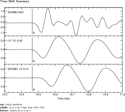
Time-Shift

There is no function in SAC that time-shifts a waveform, but as mentioned in the help file lowpass for the low-pass filter command, such filters time-shift the data, and one may want to correct for that time shift. One can use SAC to time-shift a waveform by changing the "b" header value for the SAC file. A (new as of v102.0) macro: ${SACHOME}/macros/sac-ts.m is an example of how to do this.

A Fortran program named time_shift.f in ${SACHOME}/doc/examples/time_shift does a time shift by taking the Fourier transform of the input time series then and doing the time shift in the frequency domain. Before taking the Fourier transform the waveform is prepared by taking out the mean/trend and then tapered to stabilize the Fourier transform. It is padded with zeros to minimize wrap-around.

All steps for an example are included in which a waveform is first low-pass filtered, which results in a time shift, and that time shift is taken out by the two methods: a call to the SAC macro and a run of program time_shift. The plot below shows the original plus the two methods for time-shifting the waveform for thus case.

Convolution

Prior to SAC v102.0, the SAC CONVOLVE command was effectively the same as the SAC CORRELATE_command except for a sign change. For both the CORRELATE command and the previous version of CONVOLVE, the calculation is done in the frequency domain. The explicit method used for doing the convolution is called a "discrete" convolution. For many application that method is appropriate, but a discrete convolution has two features that potentially are undesirable when applied to time series:

• no scaling of the output by the digitizing interval, and
• no check on the start time for the pulse.

The more serious problem is the second one: If the "pulse" is centered at time zero, the old SAC CONVOLVE gave an incorrect waveform.

The directory ${SACHOME}/doc/examples/convolve has both FORTRAN and C programs with options for both discrete convolution and "time-series* convolution, which treats convolution for a time series "correctly".

Sample Runs

Input for the convolution can be generated as:

SAC> fg triangle npts 8 delta 0.02 begin -0.08
SAC> write triangle_n8_d0.02.sac
SAC> fg impulse npts 12 delta 0.02 begin 0
SAC> write impulse_n12_d0.02.sac

Then run the convolvef program:

% ./convolvef
Usage: convolvef p_name wf_name c_name disc_conv
  where the first three arguments are filenames
  for pulse, waveform, and convolution output.
If disc_conv is y, it uses a discrete convolution
  and the pulse begin time is set to zero.
If disc_conv is n, pulse begin time is unchanged
  and the output is multiolied by delta, which is
  what one has in a time-series covolution.
% ./convolvef triangle_n8_d0.02.sac impulse_n12_d0.02.sac conv_y.sac y
% ./convolvef triangle_n8_d0.02.sac impulse_n12_d0.02.sac conv_n.sac n

The pulse file triangle_n8_d0.02.sac is symmetric around zero time, so comparing the last argument "y" and "n" for disc_conv demonstrates an important difference between discrete and time-series convolutions.

Convolution Primer

In these application, f, is a waveform time series that is convolved with a pulse g. The equation for their convolution is

Both f and g are functions of time, and their zero times are coupled through the term g(t-t'). From the above equation, it is easy to show that one can choose the time zero for y and f to be the same. In the applications discussed below, the zero time for g(t) can be the same as or less than the zero time for f(t).

To calculate the convolution, one discretizes both f and g and replaces the integral with a sum. In this discussion \(\delta t= 0.02 s\) is the digitizing interval for y, f, and g. One multiplies the sum by \(\delta t\), which is not what is done in a discrete convolution, which also does not take into account any difference in zero time between f(t) and g(t).

Here, two applications of convolution are discussed. Both have the same f(t) but different g(t).

f(t) is a synthetic waveform (produced using Haskell matrices or WKBJ) where vertical lines of calculated polarities and amplitudes are drawn at phase-arrival times. For these examples, the synthetic waveform is a vertical-component time series for an incident P-wave at an angle of \(20^\circ\) with the vertical through a 2-layer crust. There are \(n_w = 2048\) points in the discretized f. (The large number is chosen to minimize wraparound.) The duration is \(t_w = \delta t [n_w-1]\). The first point in f is chosen to be at t = 0, so \(f(t) =f(t)H(t)H(t_w-t)\),where

g(t) is a pulse waveform with a far smaller duration than f(t). Here, the pulse is either (1) an approximation of a P arrival so that the output of the convolution potentially models the data, or (2) a time-symmetric shape with a maximum at t = 0 to smooth out the Gibbs phenomenon that often accompanies arrivals in synthetics. Option (2) is often used for synthetics for receiver functions.

A “Brune” pulse for (1): \(g(t) =U_0 H(t) t e^{-t/\kappa} H(t_p-t)\), where \(\kappa=0.1 s\), \(t_p=1.26 s\), and \(U_0\) is a constant that only affects the amplitude, so is of no interest here.

For (2), the source pulse is a triangle function produced by fg in SAC:

fg triangle npts 8 delta 0.02 begin -0.08.

Note that the Brune pulse starts at the same time as f, while the triangle pulse starts at a negative time with a maximum at the start time for f. If the total time for the pulse is \(t_p\) , the general form for the pulse is \(g(t) =g(t)H(t-t_1)H(t_2-t)\), where for the Brune pulse \(t_1=0\), \(t_2=t_p\) and for the triangle pulse \(t_1=-0.08s\), \(t_2 = 0.06s = t_p-t_1\). For either pulse, \(t_p=\delta t[n_p-1]\).

Given the above forms for f and g , the original convolution equation can be written

For the Brune pulse, \(t_1=0\), so t cannot be negative, but for the triangle pulse the lower bound for t is -0.06 s. In Fortran, arrays are stored in the computer using positive integers, so to simplify the bookkeeping it is best to avoid negative times when we discretize the above equation. One can avoid negative times if one chooses \(y(\tau) =y(t-t_1)\). With this choice the modified equation then reads

The discretized equation for the above is then

where \(j_1 = -(t_1/\delta t) + 1\) and i runs from 1 to \(n_w + n_p - 1\)

The following Fortran code produces the correct result for the convolution for either pulse

j_1 = -nint(b_p/delta)+1
do i=1,n_w+n_p-1
  temp = 0.0
  do j=1,n_w
    if (i.ge.(j-j_1) .and. n_p.ge.(i-j+j_1)) then
        temp = temp + waveform(j)*pulse(i-j+j_1)
    endif
  end do
  conv(i) = delta*temp
end do

where \(b_p = t_1\), delta = \(\delta t\), and conv(i) = \(y_i\).

Plots for the two pulse waveforms are shown in Figure 1, and the results of the convolution near the first synthetic arrival are shown in Figure 2 both for the Brune pulse and for the triangle pulse. The Gibbs phenomenon is quite pronounced at the arrival in the raw synthetic. Note that the peaks for the arrival in Figure 2 are at the same time for the triangle-pulse convolution and the synthetic, and the Brune-pulse convolution starts at the peak of the raw-synthetic arrival time. For display purposes, the waveforms are time-shifted so that the first arrival are at five seconds into the record. Hence the zero time for the display and the convolution calculation are not the same.

If one uses the SAC convolution for the two runs, one gets the "correct" result for the Brune pulse but a time shift of 0.08 seconds for the triangle pulse (which starts at -0.08 s). The convolution of the triangle pulse with itself is also time-shifted 0.08 s. If one uses the SAC CONVOLVE option "amplitude on" in program convolvef or convovlec, one gets the same amplitudes and times as for the discrete convolution output.

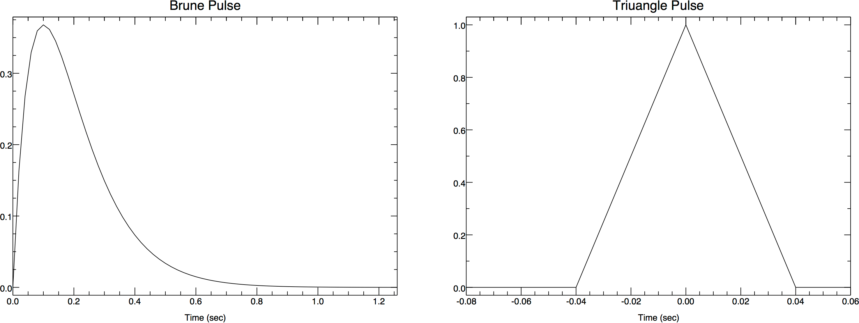
Figure 1. The two source pulses used for these convolution applications.

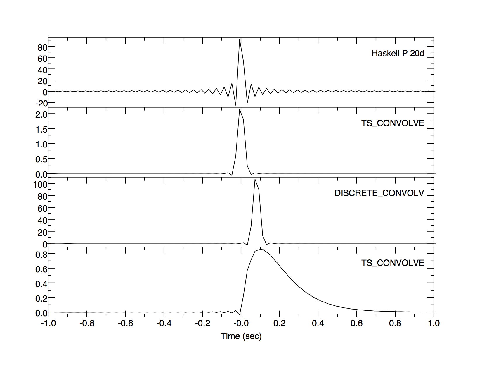
Figure 2: From top to bottom: unfiltered synthetic, time-series convolution with triangle pulse, discrete convolution with triangle pulse, time-series convolution with Brune pulse